
Accurate analyte concentration determination is a cornerstone of analytical chemistry. Particularly in applications involving environmental monitoring, biological research, and industrial quality control. Traditionally, a calibration equation serves in determining the unknown concentration of an analyte by measuring a sensor’s response to a series of known standards. However, when working with complex sample matrices—such as biological fluids, soil extracts, or solutions containing heavy metals—the direct comparison between the sample and standard solutions becomes problematic due to the matrix effect. The matrix effect occurs when interfering substances within the sample alter the instrument’s response. Thus, leading to inaccuracies in the calculated analyte concentration. To counteract this issue, chemists use the standard addition procedure. This is a technique that enhances measurement accuracy by compensating for matrix effects while still leveraging traditional calibration principles.
Why Use the Standard Addition Procedure?
The standard addition method, also known as spiking, improves the accuracy of analyte concentration measurements in heterogeneous or complex samples. Instead of relying on a separate calibration curve, this approach involves adding known amounts of the analyte directly into the sample. Therefore, allowing the instrument to detect changes in response solely due to variations in analyte concentration.
By analyzing these response shifts, researchers can calculate the true concentration of the analyte while accounting for interfering substances within the sample matrix. This makes the standard addition method particularly useful in applications where sample composition is unknown or highly variable, such as:
- Pharmaceutical testing – Measuring drug concentration in blood plasma or urine.
- Environmental monitoring – Detecting heavy metals in river water or soil samples.
- Food safety analysis – Identifying contaminants in processed foods or beverages.
How the Standard Addition Procedure Works
Step 1: Preparing Test Solutions
Prepare a series of test solutions, each containing equal volumes of the sample (Vx) with an unknown concentration (Cx). Also, add increasing amounts of analyte standards (Vs) with a known concentration (Cs) are to each test solution. Except for one control solution, which contains only the sample and solvent.
By gradually increasing the concentration of the analyte in successive test solutions, scientists can observe how the sensor’s response changes with each addition. This step is crucial for distinguishing the analyte’s signal from interfering substances in the sample matrix.
Step 2: Measuring Instrument Response
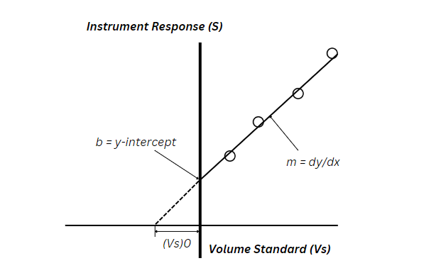
Once the solutions are prepared, the instrument measures the sensor response (S) for each test solution. Thereafter, generating a series of response values corresponding to the increasing concentrations of the analyte. The collected data is then plotted on a calibration graph, where:
- The x-axis represents the spiked volume of the analyte standard (Vs).
- The y-axis represents the sensor’s response (S) to each solution.
This graph forms a linear calibration curve, showing how the signal increases as more of the analyte is added.
Step 3: Calculating the Unknown Concentration
A linear regression analysis is performed on the plotted data, resulting in the equation:
![\[ S=mV_{S}+b\; \; \left [ Equation1 \right ] \]](https://alpha-measure.com/wp-content/ql-cache/quicklatex.com-a8fdf9b18fbfbef44b8d20f35dce7eb3_l3.png "Rendered by QuickLaTeX.com")
The procedure relies on the assumption that the instrument response would drop to zero if no analyte were present. This assumption helps in determining the original analyte concentration in the sample. Also, by extrapolating the calibration curve to the point where the response reaches zero, scientists identify the equivalent volume of the standard needed to compensate for the analyte present in the sample.
The unknown analyte concentration Cx can be determined using the equation:
![\[ c_{x}=\frac{bc_{s}}{mV_{x}} \]](https://alpha-measure.com/wp-content/ql-cache/quicklatex.com-af156d8303c06a4650aee728da9d3e9c_l3.png "Rendered by QuickLaTeX.com")
where:
- Cx is the concentration of the analyte in the sample.
- Cs is the known concentration of the standard.
- b is the y-intercept of the calibration curve.
- m is the slope of the calibration curve.
- Vx is the volume of the sample aliquot.
This calculation allows for an accurate determination of the analyte concentration while minimizing errors caused by matrix effects.
Advantages of the Standard Addition Method
In comparison to traditional external calibration, the standard addition procedure offers several benefits:
- Compensates for Matrix Effects – By adding the analyte directly to the sample, the method eliminates discrepancies. These discrepancies are usually due to unknown or interfering substances.
- Improves Accuracy in Complex Samples – Useful for biological fluids, environmental samples, and industrial solutions where composition is unpredictable.
- Eliminates Need for Identical Standards – Unlike traditional calibration methods, standard addition does not require that standards and samples share the same solvent or background matrix.
- Reduces Measurement Variability – All measurements utilize the same sample. Hence, minimizing variations due to sample handling or instrument drift.
However, the technique does have some limitations. Standard addition requires multiple measurements, increasing experimental time and reagent consumption. Additionally, for high-precision applications, careful pipetting and accurate volume control are essential to minimize errors in the standard additions.

